Shapefiles

Shapefiles

Valley Bottom

How to:

1. Create a polygon shapefile named valley_bottom.shp

2. Fields:

   area_sq_m - type decimal (double)

   date - type date

   waterbody - type string

3. Digitize the valley bottom

4. Use the “Smooth” tool at default values

5. Remove your old valley_bottom layer from the map and export the new “Smooth” temporary layer, overwriting your old shapefile. Keep the name as valley_bottom

6. Field calculate necessary fields

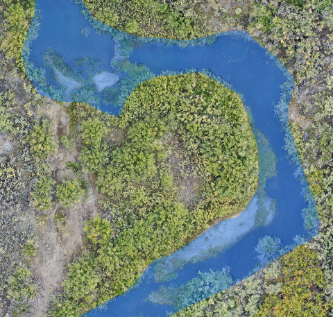
What is this layer? Valley bottom is the stream/river channels and the nearby low-lying contemporary floodplain. The spatial extent of the valley bottom is defined as the area that could plausibly flood during the contemporary flood regime. THIS SETS THE EXTENT OF YOUR DIGITIZING. None of the remaining shapefiles from this point on should exceed your valley bottom. In some instances the drone imagery may not include enough of the lateral extent of the valley bottom. In these cases it is okay if your valley bottom is wider than the ortho, just use some other imagery to help you. Remember: the valley bottom sets the extent of your digitizing not the orthoimage.

Lines of Evidence:

In sufficiently resolved elevation rasters such as ones derived from drones you may see a “lip” where the elevation changes from flatter valley bottom to steeper hill slopes rapidly.

You may see a change from dense vegetation to sparse vegetation because slope is too steep to support vegetation.

If there is a VBET run for your area, that is also a good line of evidence

Images:

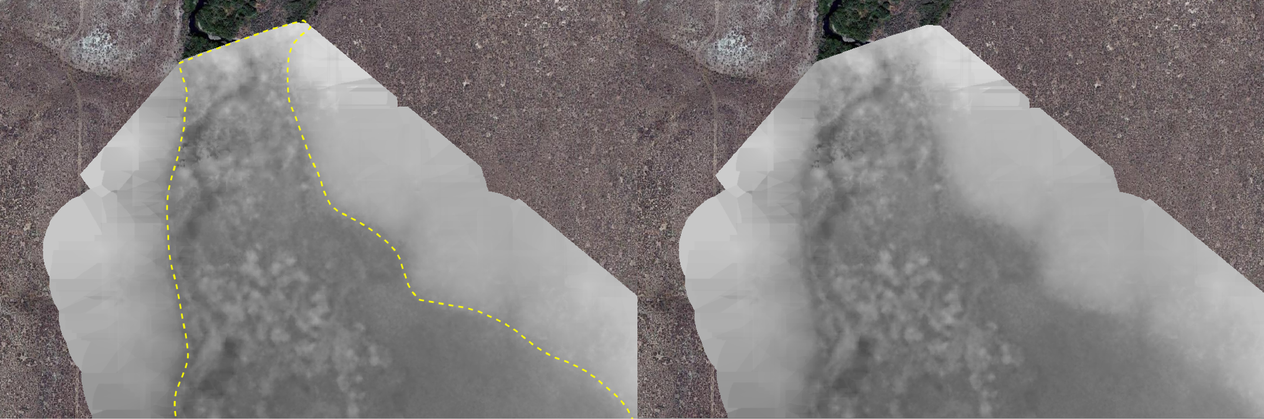
Valley Bottom Centerline

How to:

1. Create a line shapefile named vb_centerline.shp

2. Fields: None

3. Use the polygons to lines tool on the valley bottom shapefile

4. Use the locate points along lines tool from the plugin and input the “Lines” temporary file you just created. Offset 0, interval 1, give it an output name, check the “Add Vertices” box, then run.

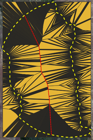
5. Use this new points temporary layer as the input for the “Voronoi polygons tool”

6. Using the snapping and trace tools in QGIS, digitize the line that runs down the center of the valley bottom.

What is this layer? This line shows the center of the valley bottom. This can be used in conjunction with ac_centerline to determine sinuosity. It’s useful for data processing after digitizing

Lines of Evidence:

Voronoi polygons layer

Images:

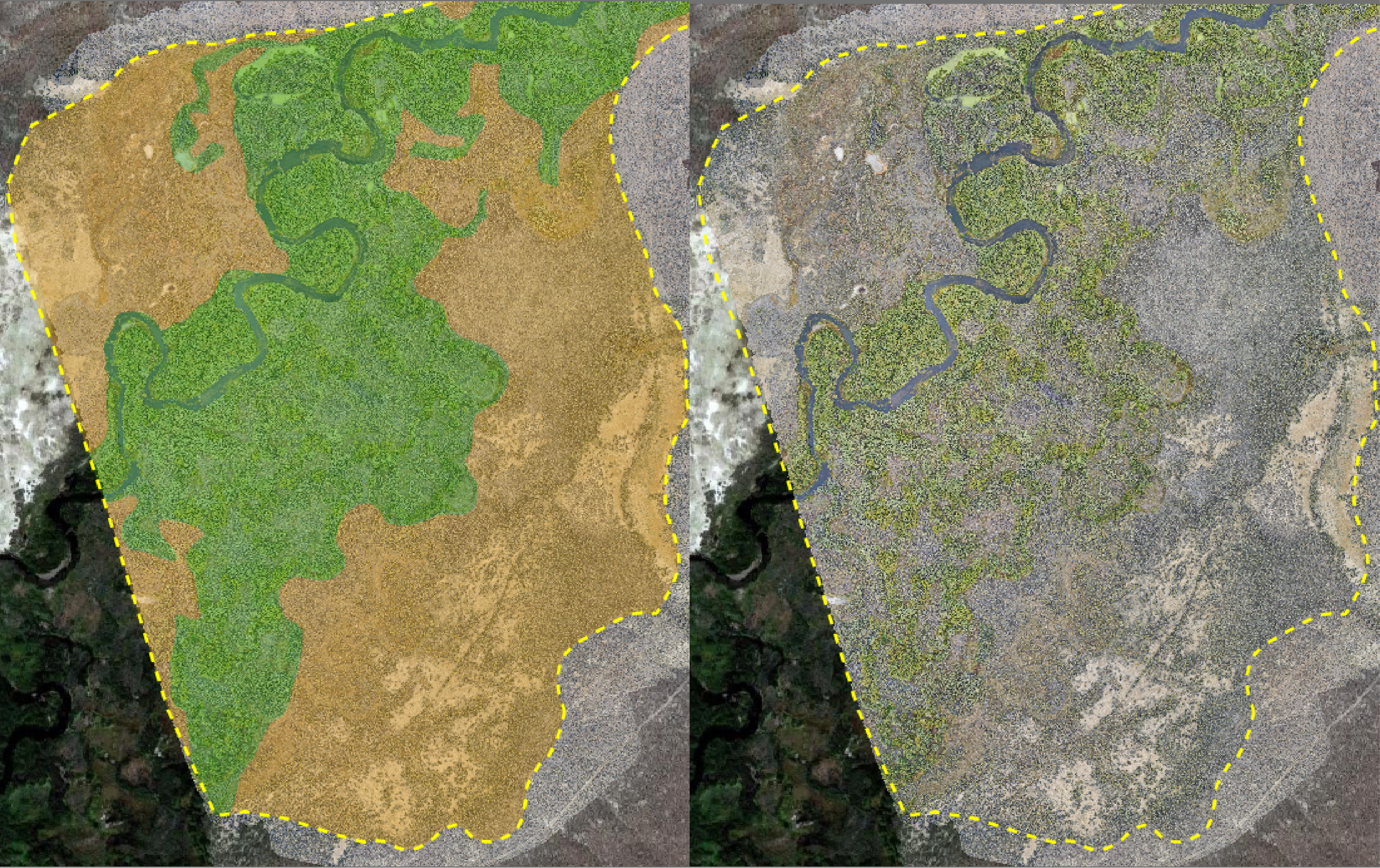
Riparian

How to:

1. Create a polygon shapefile named riparian.shp

2. Fields:

   area_sq_m - type decimal (double)

   type - type string

   • riparian
   • upland

   date - type date

   waterbody - type string

3. Copy and paste the valley bottom polygon into the Riparian shapefile, for the type, fill in “upland”

4. Digitize the riparian areas and for these polygons enter the type as “riparian”, ensure trace is enabled for areas that abut the valley bottom.

5. From here, select all the areas labeled as riparian and then clip them from the upland polygon by clicking the “Clipper” icon from the clipper toolbar. (You can also do riparian in step 3 and then upland in step 4, do what makes more sense)

6. Calculate fields

What is this layer? The riparian layer is our approximation of the floodplain. Previously we had tried to map floodplain but the lines of evidence were weak. Now we map riparian as a way to approximate the current floodplain without making any false claims as to where the floodplain may really be. This layer delineates upland plants vs. riparian plants.

Lines of Evidence:

Perennial riparian vegetation

In desert systems riparian can sometimes be the only greenery in the valley bottom

If the riparian stands are dead, this does not count as riparian

Suppression of upland vegetation growth indicates riparian

NDVI raster if available

Images:

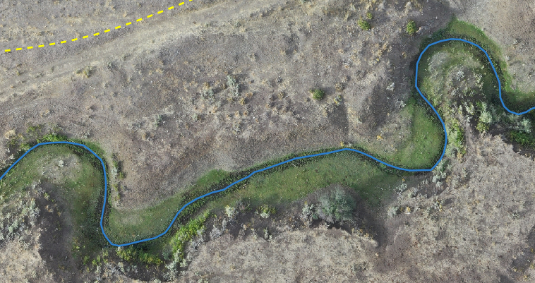
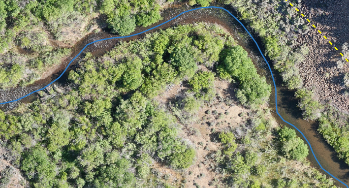
Active Channel

How to:

1. Create a polygon shapefile named active_channel.shp

2. Fields:

   area_sq_m - type double

   date - type date

   waterbody - type string

3. Digitize the channel edge, this includes bars and islands that are in the channel

4. Calculate fields

What is this layer? Active channel is the area of the channel that is modified by average stream discharge. This means it includes non wetted features such as islands and bars that are located within the bankful channel.

Lines of Evidence:

Clear signs of scouring

Channelization

Bars

Elevation raster may show the channel

Breaks in the tree line

Greener areas beside the channel

Generally no non-aquatic vegetation, in non-perennial systems there may be some grasses growing in the channel during the dry season

Images:

Active Channel Centerline

How to:

1. Create a line shapefile named ac_centerline.shp

2. Fields: None

3. Use the polygons to lines tool on the active channel shapefile

4. Use the locate points along lines tool from the plugin and input the “Lines” temporary file you just created. Offset 0, interval 1, give it an output name, check the “Add Vertices” box, then run.

5. Use this new points temporary layer as the input for the “Voronoi polygons tool”

6. Using the snapping and trace tools in QGIS, digitize the line that runs down the center of the active channel.

What is this layer? This line shows the center of the active channel. This can be used in conjunction with vb_centerline to determine sinuosity.

Lines of Evidence:

Voronoi polygons layer

Images:

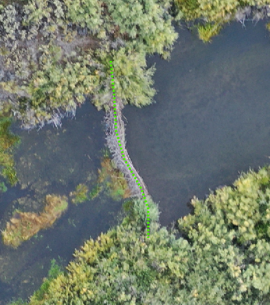
Dam Crests

How to:

1. Create a new line shapefile named dam_crests.shp

2. Fields:

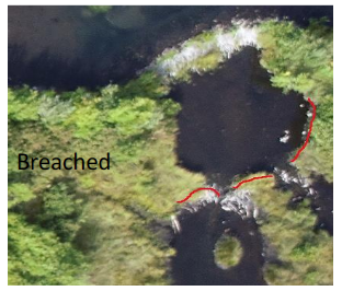
   dam_state - type string

   • intact
   • breached
   • blown_out

   date - type date

   waterbody - type string

3. Trace the crest of each observed dam, in cases where the dam has damage, trace where the crest would be if it was intact

4. Calculate fields

What is this layer? This layer traces the top crest of a dam to show location, extent, and state of the dam. The options for dam_state are intact, where the dam is intact, breached, where the dam has some damage but is still ponding water at a lowered level, and blown_out where there is structural damage the whole height of the dam so it is not ponding water. Ponded water should be traced along the dam crest line if a dam crest is present, then the free flowing after should trace that same dam crest line.

Lines of Evidence:

Ponded water

Dams are generally convex with the current

Does the dam have a mattress? A mattress is branches that lay on the downstream side of a dam parallel to the current to help dampen the strength of any overflow and prevent scouring at the base of a dam.

Be careful to make sure this isn’t a woody debris accumulation.

“Bath tub” ring of mud around the perimeter of the dam indicating a relatively recent breach

Area of concentrated flow at the location of the breach

Images:

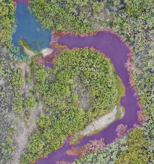
Inundation

How to:

1. Duplicate the active_channel layer by exporting it and saving as inundation.shp. If you prefer you can make a polygon from scratch rather than reshaping and building on the active_channel shapefile.

2. Fields:

   type - type string

   • free_flowing
   • ponded
   • overflow

   area_sq_m - type double

   date - type date

   waterbody - type string

3. Using the reshape and add ring tools, modify the polygon to fit where there is water. This is also a good place to use clipper or split features tools because each of these inundation types is mutually exclusive.

4. Calculate fields

What is this layer? This layer shows where the water is within the valley bottom. Free flowing is water that is flowing in the channel unobstructed, ponded is water that is being ponded by some sort of structure, generally a beaver dam, overflow is water that is being structurally forced onto the floodplain and out of the channel, or a structurally forced secondary channel.

Lines of Evidence:

Are there surrounding structures that may be affecting the flow?

Is there water in the system?

Dams can back up water much further than you may expect.

Images:

Thalwegs

How to:

1. Create a line shapefile named thalwegs.shp

2. Fields:

   type - type string

   • primary
   • secondary

   length - type double

   date - type date

   waterbody - type string

3. Digitize along the deepest part of the channels you’ve previously digitized, ensure snapping is enabled so that thalweg segments connect to each other

4. Calculate fields

What is this layer? This layer delineates the deepest part of the channel for the whole length of the channel. The primary thalweg is the thalweg that runs through the main channel, secondary thalwegs run along side channels and areas where the primary thalweg may split due to structures in the stream or islands.

Lines of Evidence:

Look for areas in the channel that appear darker, these are likely deeper water than the surrounding channel

In systems that are dry or drying, whatever remaining water is in the channel likely follows the thalweg

The primary thalweg is the thalweg in the larger channel, if there are two channels that are similar sizes, use the channel that follows the google maps trace of the river and has a name.

Images:

Confluences and Difluences

How to:

1. Create a point shapefile named confluence_difluence.shp

2. Fields:

   type - string

   • D
   • C
   • C/D

   date - type date

   waterbody - type string

3. Digitize c/ds where there are thalwegs that meet and split

4. Calculate fields

What is this layer? This layer maps flow patterns in a channel. Confluences are where water meets and difluences are where water splits. C/D can be used where one area has both a difluence and a confluence, you can also place a C and a D point at these places if that makes more sense to you rather than one C/D point.

Lines of Evidence:

Thalwegs converge or diverge

Islands

Determine flow direction by looking at channel heads and slope. Higher elevation is generally upstream and channel heads generally point upstream.

Images:

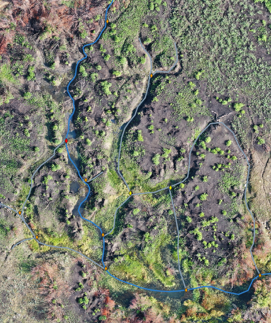
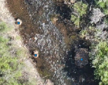
Structures

How to:

1. Create a point shapefile named structures.shp

2. Fields:

   type - type string

   • live
   • inorganic
   • jam
   • lwd
   • BDA
   • PALS

   date - type date

   waterbody - type string

3. Digitize features by placing points atop structures where you observe them.

4. Calculate fields

What is this layer? This layer can contain low tech restoration structures and other structures that are structurally forcing flows. This means that flows in some way are being modified by these structures, modification of course exists for every size of structure down to a grain of sand if you get pedantic however, for the sake of digitizing flow modification should be visible from aerial imagery. This can include bank erosion, new channels, split flows, pond formation, etc. Which set of structures you digitize may be project specific but generally digitize them all and then apply either the structures symbology or restoration structures symbology. Live means vegetation growing in the channel, inorganic can be things like boulders or tires, a jam is woody debris that is channel spanning and ponding water, lwd is large woody debris in the channel such as a fallen tree, BDAs or beaver dam analogues are human made structures meant to mimic the function and form of a beaver dam, PALS or post assisted log structures are logs being held in the channel by posts, PALS are also made by humans. Dams are should not be digitized in this shapefile because they are already digitized in dam_crests.

Lines of Evidence:

Structurally forced flows

Signs of geomorphic modification

PALS may have small circles in the structure visible from aerial imagery, those are the posts

Shapefile indicating location of LTPBR structures

Images: